How to Use INDEX and MATCH for Flexible Lookups in Google Sheets

Introduction

Are you looking for a dynamic duo that can tackle complex lookups in Google Sheets? Look no further than the INDEX and MATCH functions. Together, they form a versatile combo that outperforms VLOOKUP in many scenarios. In this tutorial, we'll explore how to use INDEX and MATCH to find data in your sheets effectively.

What Are INDEX and MATCH?

INDEX and MATCH are two separate functions in Google Sheets that, when combined, allow you to look up values both vertically and horizontally. This flexibility makes them a valuable tool for data analysis.

The INDEX function

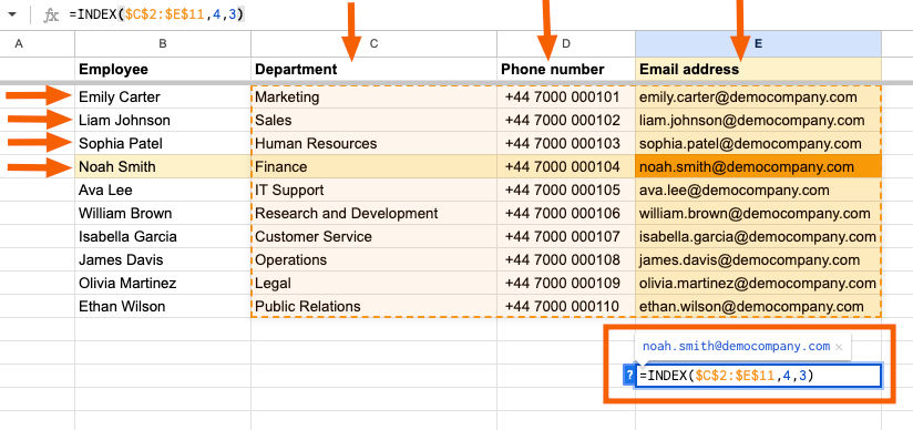
The INDEX function returns the value of a cell in a specified row and column within a range. For example, in its simplest form, we can index this table and ask for the value four rows down and three columns across; this gives us the email address for the employee Noah Smith.

The MATCH function

The MATCH function searches for a specified item in a range and returns the relative position of that item. For example, taking the example below and using the MATCH function to look for the search key; we’re looking for Noah Smith, and we want to know its position. 

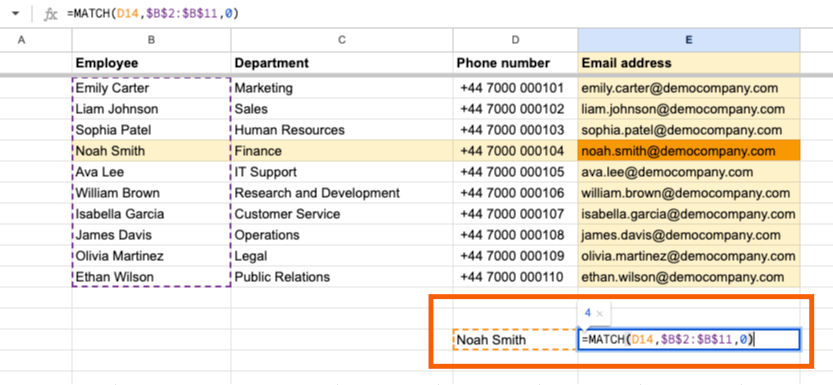
The function simply looks at each value in the range and compares it to the search value. When they match, the position is provided. Emily Carter is in position 1, Liam Johnson in position 2, Sophia Patel in position 3 and finally, Noah Smith is in position 4, which matches the search key; therefore, the value of 4 is returned. 

How Do They Work Together?

When combined, INDEX and MATCH can look up a value at the intersection of a certain row and column in your data range. This makes them perfect for situations where VLOOKUP falls short, especially when you need to search to the left or perform horizontal lookups; the former is not possible with a VLOOKUP, but the latter is achievable with a HLOOKUP function. 

Essentially, we’re replacing the INDEX row and column values with a MATCH function. In the example above, we asked for row four in the INDEX function like this:

=INDEX($C$2:$E$11,4,3)

Then, in the second example, we looked for a specific name and returned the position of this value with the MATCH function, giving us a value of 4, like this:

=MATCH(D14,$B$2:$B$11,0)

We can just replace this row position (4) of the index with the MATCH, like this:

=INDEX($C$2:$E$11,MATCH(D14,$B$2:$B$11,0),3)

We can do the same for the column position, too, to return a value of 3, like this:

=MATCH(D15,$C$1:$E$1,0)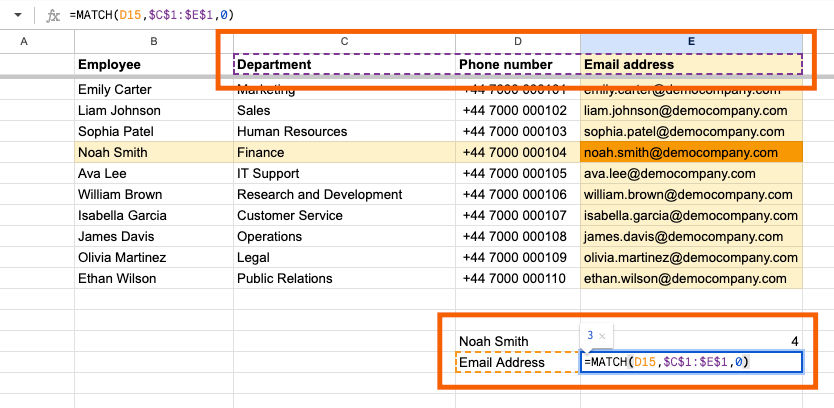

The final formula will look like this below, and we’ll retrieve the highlighted email address from the table. 

=INDEX($C$2:$E$11, MATCH(D14,$B$2:$B$11,0), MATCH(E13,$C$1:$E$1,0))

If you look closely, you’ll see we simply replaced row 4 in the INDEX function with the ROW MATCH function, and column 3 in the INDEX function with the COLUMN MATCH function.

Here’s the final formula again, the INDEX part remains largely the same, but the row position 4 is replaced with the MATCH function (highlighted yellow) below, and the column position 3 is replaced with the MATCH function (highlighted green) below.

=INDEX($C$2:$E$11,  MATCH(D14,$B$2:$B$11,0), MATCH(E13,$C$1:$E$1,0) )

Practical Example

Suppose you had a huge dataset where you wanted to locate a particular value, and you know two lookup values. It’s possible to construct a dynamic lookup using this INDEX and MATCH setup to locate any value with the help of drop-down menus. 

This example below uses the same function shown above, but the lookup values for the employee name and the column are now conveniently stored as drop-down menus to make this a breeze. 

Here is the formula for that, with the image below showing the ranges and lookup cells.​​

​​=INDEX($C$2:$E$11,MATCH(D14,$B$2:$B$11,0),MATCH(E13,C1:E1,0))

This returns the value of Human Resources in lookup column C (Department) for the employee name Sophia Patel. By asking the function to search for Sophia Patel in the department column, it returns the value in that position. This is 3 rows down in column 1 of the lookup range. Which is the same as performing a simple INDEX like this:

=INDEX($C$2:$E$11,3,1)

Conclusion

With INDEX and MATCH, you CAN unlock a new level of flexibility in your data analysis tasks. They may seem complex at first, but once you get the hang of them, you'll appreciate their power and versatility.

If you want to have a practice yourself, you can make a copy of this demo sheet here. All the examples have been broken down step by step so you can see the process of constructing an INDEX function through to a dynamic INDEX and MATCH function. 

If you like this, you should also add the XLOOKUP to your repertoire.

Just one final point to make about the MATCH function is the final zero, which is the search type. The search method is 1 by default, which finds the largest value less than or equal to search_key when the range is sorted in ascending order. 0 finds the exact value when the range is unsorted. -1 finds the smallest value greater than or equal to search_key when the range is sorted in descending order.

MATCH(search_key, range, [search_type])

Generally speaking, you’ll always want to set this to zero, just as you’ve seen in these examples. It’s the safest option for returning the exact match in scenarios like this.