6 Ways to Round Numbers in Google Sheets

Rounding in Google Sheets seems simple, until it isn’t.

You might start with something straightforward like a ROUND function:

=ROUND(A1, 2)

But then, real-world scenarios creep in:

• You need prices that always end in .99

• You can’t under-order stock

• You only want to bill completed 15-minute intervals

• You’re rounding to the nearest £0.05, not decimal places

Suddenly, ROUND isn’t enough, and that’s where most people get stuck.

The problem is, Google Sheets doesn’t just have one way to round numbers; it has numerous functions that behave very differently:

• Some round to the nearest value

• Some always round up 

• Some round down

• Some round to multiples instead of decimal places

And if you use the wrong one, you can end up quietly introducing errors into your reports, or just not getting what you want. 

The key insight

There aren’t just “different rounding formulas”, there are different types of rounding:

• Direction-based for rounding up, down, or to the nearest

• Precision-based for rounding to decimal places vs multiples

• Intent-based to round for pricing, billing, inventory, and reporting, etc.

Once you understand this, choosing the right function becomes obvious. In this post, we’re going to explore the options to unveil the mysteries and bring clarity to rounding in Google Sheets. 

Stick around to discover which rounding formula works best for each scenario. You’ll be surprised, so keep reading.

The six functions you actually need

There are more than 10 rounding-related functions in Google Sheets, but these six cover almost everything, so let’s jump in and take a look at what you need, starting with the basic ROUND function. 

1. ROUND - Standard rounding

=ROUND(value, places)

This function rounds a number to the decimal places you define with the ‘Places’ argument. It has two arguments, but ‘places’ is optional.

Value

The value to round. This can be a number or a cell reference.

places - [optional]

The number of decimal places to round to.

Use when you want normal rounding (up or down).

Example: Reporting

=ROUND(B3,2)

In this example, the second argument ‘Places’ is set to ‘2’, so the result has two decimal places. This function rounds to the nearest value.

The ROUND function is generally best for:

• Generic rounding in reports

• Dashboards

• Cleaning decimals

2. ROUNDUP - Always round up

=ROUNDUP(value, places)

Rounds a number to a specified number of decimal places, consistently rounding up to the next valid value.

Value

Always round up the value to the specified number of 'places'.

Places - [optional]

The number of decimal places used for rounding.

Use when: It's important not to underestimate.

Example: Ordering stock

=ROUNDUP(I5/10, 0)

Best for:

• Inventory

• Billing

• Resource planning

3. ROUNDDOWN - Always round down

=ROUNDDOWN(value, places)

Rounds a number to a specified number of decimal places, consistently rounding down to the nearest valid increment.

Value

Always round down to the specified 'number' of decimal places.

Places - [optional]

Specifies how many decimal places to round to.

Use this when you prefer conservative values.

Example: Budget control

=ROUNDDOWN(H5, 2)

Best for:

• Budgets

• Estimates

• Limits

4. MROUND - Nearest multiple

=MROUND(value, multiple)

Rounds a number to the closest integer multiple of another. Don’t worry, we’ll explore what this means in a moment. 

Value

The number to be rounded to the closest integer multiple of another number.

Factor

The value to which the multiples will be rounded.

Use this when working with fixed increments.

Best for:

• Retail pricing

• Time intervals

• Batch sizes

Factors or Multiples

Multiples are a concept most people struggle with. Decimal rounding is what most people expect, for example, in this example, you’re saying: “Keep 2 decimal places”

=ROUND(H3, 2) - Result 12.83

Rounding to multiples is a completely different idea, and this is where things can often get confusing.

Example: Pricing to the nearest £0.05

=MROUND(B3, 0.05)

With multiples, you’re saying: “Find the nearest multiple of 0.05”

That means Google Sheets will choose between:

• 12.80

• 12.85

  
  

Result: 12.85

Another way to think about it, multiples are fixed steps on a number line.

• 0.05 - steps of 5 pence or 5 cents

• 1 - whole pounds or dollars

• 15 minutes - time blocks

• 6 - pack sizes

You’re not controlling decimals; you’re controlling which values are allowed as results. 

Here is an example of rounding a duration to the nearest 15 minutes. Remember, MROUND does not always round up;  it rounds to the closest 15-minute mark.

We’ll explore how this TIME function works a bit later, so keep reading. 

5. CEILING - Round up to a multiple

An important distinction to note, both MROUND and CEILING round a number to a specified multiple, but MROUND chooses the nearest multiple, while CEILING always rounds up to the next one, regardless of proximity.

So, if you have grasped MROUND, then CEILING will be easy peasy. 

CEILING rounds a number upward to the closest integer multiple of a specified significance factor.

=CEILING(value, factor)

Use when: You must round up to the next valid increment.

Example: £x.99 pricing

=CEILING(B5,1)-0.01

Let’s break down what’s happening here. It’s a two-step process.

Step 1 -  The CEILING part of the formula is only this part:=CEILING(B5,1)...

This takes the value from cell B5 and rounds up to the closest integer multiple. In this case, 1, so 10.13 becomes 11, because 1 is a whole number; it essentially rounds up from 10 to 11. 

Step 2 - Then we just take away 0.01, so this -0.01 at the end rounds the value 11 to 10.99. In other words, 11 - 0.01 = 10.99.

Here is another example, which is helpful in pricing to round to 49 pence or cents, using the same principle as above, but with a multiple of 0.5 rather than 1. 

Best for:

• Pricing strategies

• Shipping tiers

• Capacity planning

6. FLOOR - Round down to a multiple

FLOOR is the opposite of CEILING.

• CEILING  always rounds up to the next multiple

• FLOOR  always rounds down to the previous multiple

Rounds a number down to the nearest multiple of a specified significance factor.

=FLOOR(value, factor)

Use when: Only completed increments count.

Example: Billable time

=FLOOR(B6, TIME(0,15,0))

In this example, the first part of the function refers to the value in cell B6, which is a time. The factor uses a second function called TIME, in which we specify the time format as hours, minutes, and seconds. 

In this situation, the hour is set to 0, the minute to 15, and the second to 0. This means we want to round the ‘value’ down to the nearest 15-minute increment. The result is that 10:43:15 will round down to 10:30:00, as this is the nearest 15-minute factor. 

Best for:

• Time tracking

• Usage billing

• Threshold logic

Quick comparison

To put these functions into context, here are some simple examples of what each rounding function will produce for a value of 23.52 in cell A1. 

Once you see this difference, half of the rounding confusion disappears.

Final takeaway

Most rounding mistakes don’t come from bad formulas. They come from unclear intent.

Before choosing a function, ask:

• Do I need to round up, round down, or round to the nearest?

• Am I rounding to decimal places or multiples?

Answer those two questions, and the correct function becomes obvious, but if you’re ever in doubt, use the quick comparison table above to help you decide. 

Bonus: Apply to a whole column

Array formulas can be applied to most situations, especially in these rounding examples. You can simply enter the formula once in the top cell and have it automatically apply the same logic all the way down to the bottom of your table. 

Here are three examples of an ArrayFormula. Read on to see how this works. 

=ArrayFormula(IF(F3:F="", "",FLOOR(F3:F,1)-0.01))

=ArrayFormula(IF(E3:E="", "",CEILING(E3:E,1)-0.01))

=ArrayFormula(IF(E3:E="", "",MROUND(E3:E,0.05)))

What this formula does

Instead of copying the formula down to every row, an ARRAYFORMULA does it automatically for you. In other words, an ARRAYFORMULA lets one formula work on a whole column instead of just one cell.

Without it:

You will need to write a formula in row 3, then drag it down manually to all rows in your table.

With it:

One formula handles all rows at once. Just enter a single formula in one cell and all rows below this that meet that condition will have the formula applied to it automatically. 

This is especially useful if new rows are constantly being added to your table as you won’t need to manually drag formulas down into newly added rows as the ARRAYFORMULA will do it for you.  

How to apply ARRAYFORMULA

There are two easy ways to apply an ARRAYFORMULA.

1. Type it manually (most common)

Just wrap your formula like this:

=ARRAYFORMULA(your_formula_here)

2. Use the shortcut (quick method)

Mac: Cmd + Shift + Enter

Windows: Ctrl + Shift + Enter

• Write your formula normally (without ARRAYFORMULA)

• Press the shortcut

• Sheets will automatically wrap it in ARRAYFORMULA(...)

Example

Type:

=IF(E3:E="", "", MROUND(E3:E, 0.05))

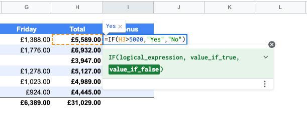
Read more on the IF Function here.

Then press:

Cmd + Shift + Enter or Ctrl + Shift + Enter

Sheets converts it to:

=ARRAYFORMULA(IF(E3:E="", "", MROUND(E3:E, 0.05)))

Master these six functions, and rounding in Google Sheets goes from confusing to completely predictable, especially once you apply a few of the practical tips and tricks along the way.

Happy rounding!